Singular Value Decomposition

SVD Theorem

For each matrix $A\in {\mathbb{R}}^{n\times m}$, there exist orthogonal matrixes $U\in {\mathbb{R}}^{\mathbb{n}\times \mathbb{n}}$ and $V\in {\mathbb{R}}^{m\times m}$ such tat $A$ can be expressed as:
$A=U\mathrm{\Sigma }{V}^T,\mathrm{\Sigma }=\text{diag}({\sigma }_1,\dots ,{\sigma }_{\text{min}\{n,m\}}),{\sigma }_i\ge {\sigma }_{i+1}\ge 0\mathrm{\forall }i$

• The set of singular values is unique
• Left/right singular vectors (columns or $U$ and $V$) can have arbitrary sign

Computation Complexity

SVD and Frobenius norm

Let the SVD of $A\in {\mathbb{R}}^{n\times m}$ be given by $A)U\mathrm{\Sigma }{V}^T$, then:
$||A|{|}_F^2=\sum _{i=1}^{minn,m}{\sigma }_i^2$

SVD and Spectral norm

Let the SVD of $A\in {\mathbb{R}}^{n\times m}$ be given by $A)U\mathrm{\Sigma }{V}^T$, then:
$||A|{|}_2:=sup\{||Ax||:||x||=1\}={\sigma }_1$

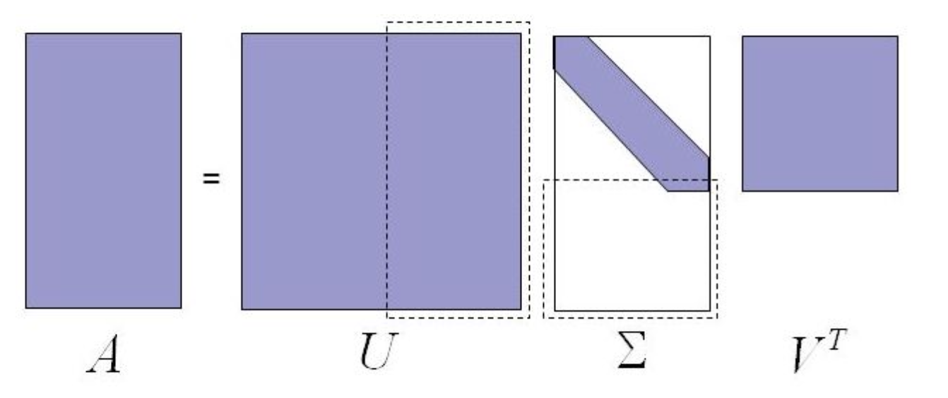
Reduced SVD

One can often prune columns of $U$ or $V$ corresponding to zero elements in $\mathrm{\Sigma }$ (or zero-padded columns/rows)

Eckart Young Theorem

• Is fundamental to many low-rank approximation problems
• This means that approximations for any $k$ can directly be read-off the SVD

Formal definition:

Corollary

The squared error of low rank approximations can be expressed as:
$||A-A_k|{|}_F^2=\sum _{i=k+1}^{\text{rank}(A)}{\sigma }_i^2$
Proof:
$A-A_k=U\text{diag}(0,\dots ,0,\dots ,{\sigma }_{k+1},\dots ,{\sigma }_{min\{n,m\}})V^T$

SVD and PCA

SVD is intimately related to eigendecomposition

• $A$ is square and symmetric: $U$ and $V$ have equal columns up to possible sign differences
• if $A$ is positive semi-definit, then the SVD is equal to the eigendecomposition
• Squares of $A$: $A{A}^T\in {\mathbb{R}}^{n\times n}$ as well as $A^{T}A\in {\mathbb{R}}^{m\times m}$:
  $\begin{array}{r}A{A}^T=U\mathrm{\Sigma }{\mathrm{\Sigma }}^T{U}^T=U\text{diag}({\sigma }_1^2,\dots ,{\sigma }_n^2)U^T\\ A^{T}A=V^T{\mathrm{\Sigma }}^T\mathrm{\Sigma }V=V\text{diag}({\sigma }_1^2,\dots ,{\sigma }_n^2)\end{array}$
  convention: ${\sigma }_r=0$ for $min\{n,m\}<r\le max\{n,m\}$

SVD and Matrix Completion

We generalize the simple rank 1 model to a rank $k$ approximation.
We do this by additive superposition of $k$ rank 1 matrices.
If all matrix entries are completely obeserved, the solution is constructively given by the SVD.

$k$ principal left singular vectors, paired with the respective right singular vector form outer products:
$A\approx \sum _{i=1}^k{\sigma }_i{u}_i{v}_i^T$

SVD with Imputation

Naive strategy:
1. estimate values for missing matrix elements (e.g. row or column mean)
2. impute them to create a complete matrix
3. run SVD to compute low rank approximation

If we have an incomplete observation, SVD is in general not applicable directly to compute low-rank approximations.

NP Hardness

Weighted Forbenius norm problem:
${\hat{A}}_k=\arg min\{\sum _{i,j}(w_{i,j}{a}_{ij}-b_{ij}{)}^2\},\text{rank}(B)=k$

• special case: $w_{ij}=w_{ij}\in \{0,1\}$, ?!!? maybe $w_{ij}=w_{ji}$
  This is NP-hard even for $k=1$