Goal: Matrix Completion
Assume we have a sparse matrix
Can we fill in the missing entries and reconstruct the matrix?
What makes a matrix a matrix (and not just a vector)?
The identity of columns and rows!
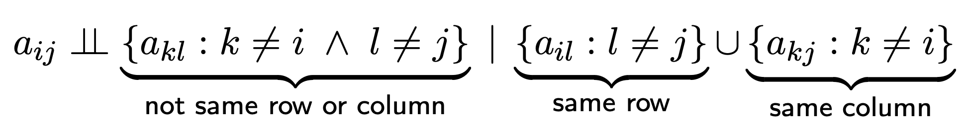
So our minimal assumption must be that entries within the same row or the same column are not independent.
We do this via conditional independence:
Recommender Systems
We analyze patterns of interest in items (products, movies) and provide personalized recommendations for users.
Collaborative Filtering
We want to exploit collective data from many users and generalize across users, and possibly across items.
Example applications are Amazon, Netflix, online advertising, etc.
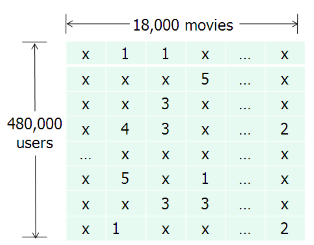
Netflix Data
Input: user-item preferences stored in a matrix
Sparseness level can be very low, 1% and less
Formal definition:
number of users (rows) number of items (columns) observation matrix, where iff is observed
Preprocessing / Normalization
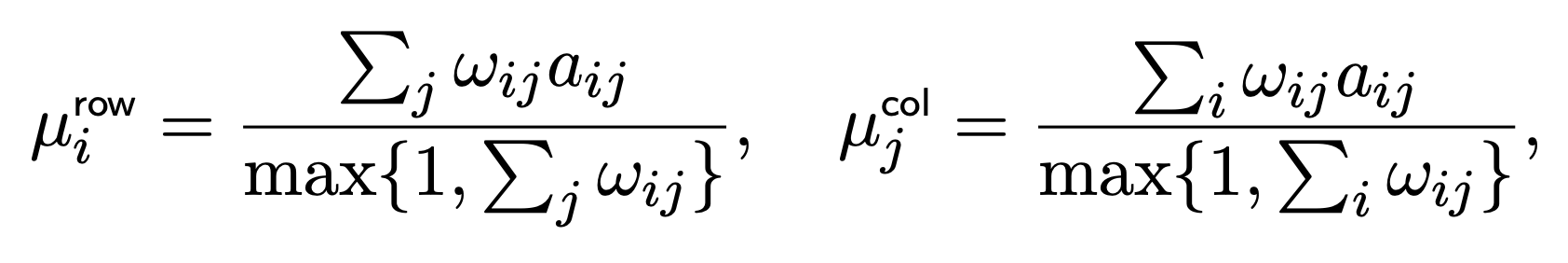
Centering
make rows/columns more comparable and subtract out rating bias
Mean rating per user/item
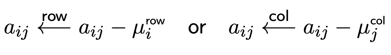
This lets us center the data:
Variance Normalization
Then the noramlized scores or z-scores are:
Convexity Definition
A set in a vector space or affine space is convex if the line segment connecting any two points in the set is also in the set
A function is convex over a domain , if for all
If is differentiable, convexity is equivalent to the condition:
if is twice differentiable, convexity on a convex domain is equivalent to the condition:
Our scalar problem is non-convex (exception: ), as there is a saddle point at the origin.
Convexity is a very fundamental property: demarcation line in optimization between tractable and (possibly) intractable problems
Gradients
Vector / Matrix notation
$\nabla_u l = Rv, \quad \nabla_vl = R^Tu, \quad R := (uv^T - A) $
Hessian Map
$ \nabla^2 l(u,v) = \left( \begin{matrix}
||v||^2 1_{n \times n} & 2uv^T - A\
(2uv^T - A)^T & ||u||^2 1_{m \times m}
\end{matrix} \right)\nabla^2 l(0,0) = \left( \begin{matrix}
0 & -A\
-A^T & 0
\end{matrix} \right)$
This is scalar to the mulitdimensional case. The hessian at zero is not positive-semi-definit , unless is nilpotent (has all zero eigenvalues).
This problem is non-convex for all dimensions
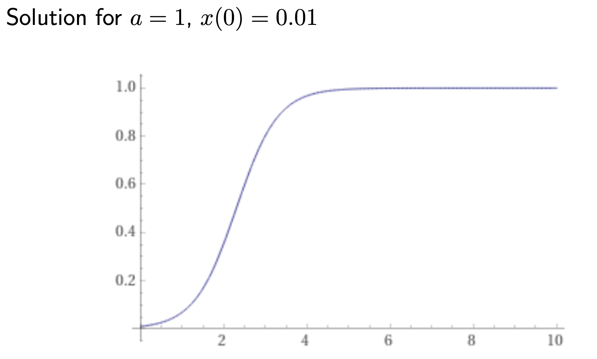
Gradient Flow
Can we gain analytic insights into the gradient dynamics?
Use ODEs to study the gradient flow = gradient dynamics in the limit of small step sizes
Assume , balanced initialization and they evolve identically.
We look at :
This ODE can be solved, yields:
Fully observed Rank 1 Model
Useful identiy:
We can then rewrite the objective:
Optimality Conditions
Directionality of is purely determined by the last term:
This can be solved with Lagrange multipliers:
First order optimality condition:
Eigenvector Equations
By putting both optimality conditions together we get the eigenvector equations: should be proportional to the principal eigenvector of should be proportional to the principal eigenvector of
Power iterations can be used for computation.